学完线性二次型问题后,我继续整理非线性轨迹优化,包括直接配点、DDP 与 iLQR 的方法和作业实践。推导部分与长代码可以分开阅读。
先修知识: LQR、动态规划、二阶泰勒展开,以及非线性动力学的数值积分。
阅读路线:
- 先区分轨迹离散化和优化求解的不同思路,理解直接配点的作用。
- 再沿值函数、局部二次近似、反向递推和前向线搜索阅读 DDP/iLQR。
- 最后按小车倒立摆、四旋翼轨迹优化和姿态调整三个案例查看实现。
笔记结合 CMU 16-745 的课程与作业整理,相关材料见课程作业页面。文中的代码片段保留学习时的实现,运行时还需使用对应作业的依赖与上下文。
Lecture 11-12 Nonlinear Trajectory Optimization/Differential Dynamic Programming
非线性轨迹优化可以采用不同的参数化与求解方式。Shooting(打靶)和 collocation(配点)不能简单地分别等同于直接法和间接法:直接打靶和直接配点都属于常见的直接方法;间接方法通常从最优性必要条件出发构造待求解方程。
直接配点把离散状态和控制作为优化变量,将动力学离散为约束,再交给非线性优化求解器。Hermite–Simpson 是常用配点方案,但不能笼统地说它在所有问题中都比 RK4 更稳定或成本更低。方法比较需结合步长、误差、问题规模和求解器。分类与直接配点可参考 MIT 的轨迹优化讲义。
注意
课程演示的代码 dircol.ipynb 在本地运行到 z_sol = solve(z0,prob) 时给出报错
ERROR: TypeError: in typeassert, expected Vector{Tuple{Int64, Int64}}, got a value of type Vector{Tuple{Any, Any}}在当时使用的接口与代码组合中,通过修改 row_col! 和 sparsity_jacobian 的索引类型处理了该错误。原记录没有完整依赖版本,这只能作为类型不匹配的排查线索,不能认定所有版本都必须改为 Int64。
row = Int64[]#而不是row=[]col = Int64[]当时执行 using MeshCat 时还遇到报错
InitError: could not load library "C:\Users\26583\.julia\artifacts\8f71eb37d5b304026b6363d835f8c65ff1920339\bin\avdevice-61.dll"The specified module could not be found.......during initialization of module FFMPEG_jll这表明 FFMPEG 动态库或其依赖加载失败,不能仅凭错误推断需要重新编译。原记录曾尝试对 FFMPEG_jll 和 MeshCat 执行 build/add,但没有保留可确认因果关系的日志,因此移除这组“一键修复”命令。
JLL 通常通过 artifacts 提供预构建二进制,Pkg.build 不是重新编译任意 JLL 动态库的通用办法。先在原作业环境记录以下信息,再根据具体缺失文件、平台支持与依赖加载错误排查;见 BinaryBuilder 的 JLL 说明。
using Pkgversioninfo()Pkg.status()# 在新 Julia 进程中单独执行 using MeshCat,并保留完整错误栈。# 不要先改动依赖版本、添加间接依赖或删除整个 artifacts 目录。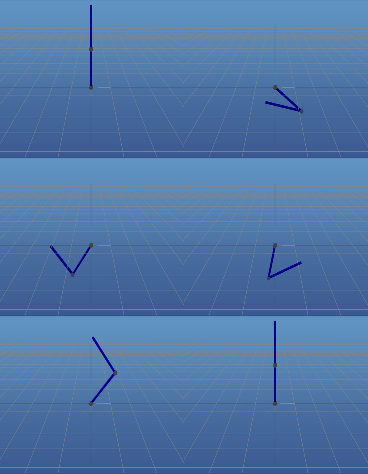
微分动态规划(Differential Dynamic Programming, DDP)是一种用于求解非线性最优控制问题的迭代算法,结合动态规划和二阶泰勒展开的思想,通过局部近似和反向传播来高效地优化控制策略。
参考文章
Differential Dynamic Programming with Nonlinear Constraints
Second-Order Differential Dynamic Programming for Whole-Body MPC of Legged Robots
考虑离散动力学系统,目标是找到控制序列,最小化总代价(通常假设代价函数和约束函数二阶可导)
DDP/iLQR:反向递推与前向更新
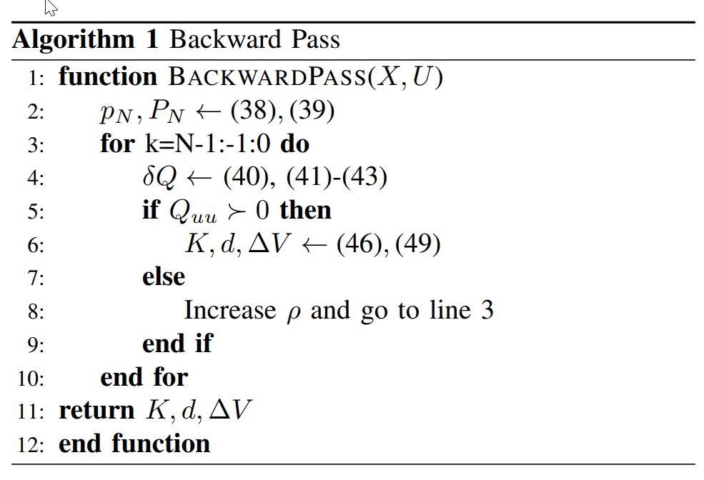
反向传播(Backward Pass)
-
定义值函数(value function)
在时间步,值函数为从状态出发,采用最优控制策略的最小总代价
-
贝尔曼方程
值函数满足贝尔曼方程(反映状态动作值函数和状态值函数的关系)
-
二阶泰勒展开
DDP 对Q 函数(即当前步代价+下一步值函数)进行二阶泰勒展开
其中
iLQR的不同在于忽略等二阶项
-
最优控制修正
固定当前状态扰动,对局部二次近似的 关于输入扰动求极小,得到控制修正(假设 正定;否则需要正则化)
其中,反馈增益,前馈增益
-
更新值函数的二次近似
其中
从开始,递推出和。
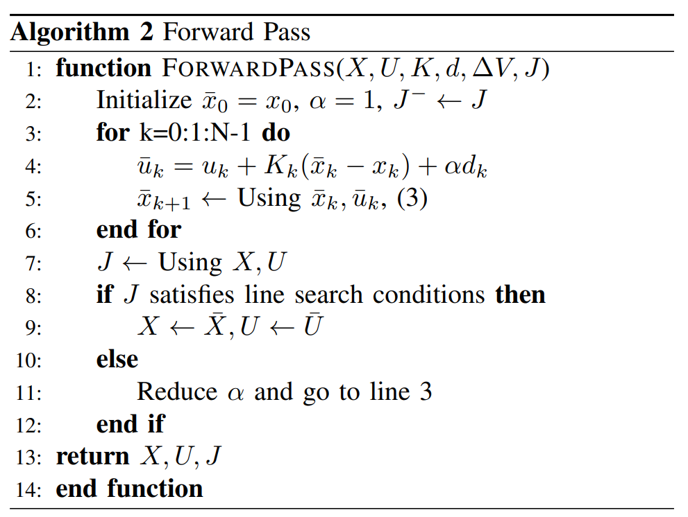
前向更新(Forward Pass)
更新控制序列
通过比较新旧轨迹代价进行线搜索,选择合适的步长 。这里统一令前馈修正 ,因此前向更新使用加号;不能把正号定义的 直接代入这一更新式。
上面的反向递推是局部无约束子问题的形式。开头列出的状态和输入约束需要额外的约束处理机制,例如增广拉格朗日;不能仅写入问题描述就认为普通 iLQR 已处理约束。参考 AL-iLQR Tutorial。
HW3_Q1 倒立摆小车DIRCOL示例
IPOPT是一个基于内点法的开源大规模非线性优化求解器,专门用于求解具有约束的连续优化问题。设定如下标准问题(这个HW自带了一个fmincon函数将IPOPT的接口进一步封装)
"""x = fmincon(cost,equality_constraint,inequality_constraint,x_l,x_u,c_l,c_u,x0,params,diff_type)
This function uses IPOPT to minimize an objective function
`cost(params, x)`
With the following three constraints:
`equality_constraint(params, x) = 0``c_l <= inequality_constraint(params, x) <= c_u``x_l <= x <= x_u`
Note that the constraint functions should return vectors.
Problem specific parameters should be loaded into params::NamedTuple (things likecost weights, dynamics parameters, etc.).
args: cost::Function - objective function to be minimzed (returns scalar) equality_constraint::Function - c_eq(params, x) == 0 inequality_constraint::Function - c_l <= c_ineq(params, x) <= c_u x_l::Vector - x_l <= x <= x_u x_u::Vector - x_l <= x <= x_u c_l::Vector - c_l <= c_ineq(params, x) <= c_u c_u::Vector - c_l <= c_ineq(params, x) <= c_u x0::Vector - initial guess params::NamedTuple - problem parameters for use in costs/constraints diff_type::Symbol - :auto for ForwardDiff, :finite for FiniteDiff verbose::Bool - true for IPOPT output, false for nothing
optional args: tol - optimality tolerance c_tol - constraint violation tolerance max_iters - max iterations verbose - verbosity of IPOPT
outputs: x::Vector - solution
You should try and use :auto for your `diff_type` first, and only use :finite if youabsolutely cannot get ForwardDiff to work.
This function will run a few basic checks before sending the problem off to IPOPT tosolve. The outputs of these checks will be reported as the following:
---------checking dimensions of everything-------------------all dimensions good---------------------------------diff type set to :auto (ForwardDiff.jl)-------------testing objective gradient--------------------------testing constraint Jacobian-------------------------successfully compiled both derivatives--------------IPOPT beginning solve----------------------
If you're getting stuck during the testing of one of the derivatives, try switchingto FiniteDiff.jl by setting diff_type = :finite.""";Part B
倒立摆小车的状态向量定义如下
求解优化问题
给定水平推力(限幅)使得倒立摆小车从到。
采用ZOH和Hermite Simpson来描述离散动力学系统,代表Hermite Simpson残差。
# cartpolefunction dynamics(params::NamedTuple, x::Vector, u) # cartpole ODE, parametrized by params.
# cartpole physical parameters mc, mp, l = params.mc, params.mp, params.l g = 9.81
q = x[1:2] qd = x[3:4]
s = sin(q[2]) c = cos(q[2])
H = [mc+mp mp*l*c; mp*l*c mp*l^2] C = [0 -mp*qd[2]*l*s; 0 0] G = [0, mp*g*l*s] B = [1, 0]
qdd = -H\(C*qd + G - B*u[1]) xdot = [qd;qdd] return xdot
endfunction hermite_simpson(params::NamedTuple, x1::Vector, x2::Vector, u, dt::Real)::Vector # TODO: input hermite simpson implicit integrator residual x1_dot=dynamics(params,x1,u) x2_dot=dynamics(params,x2,u) xm=(x1+x2)/2+dt*(x1_dot-x2_dot)/8 xm_dot = dynamics(params,xm,u) return x1+dt/6*(x1_dot+4*xm_dot+x2_dot)-x2end定义优化变量
function create_idx(nx,nu,N) # This function creates some useful indexing tools for Z # x_i = Z[idx.x[i]] # u_i = Z[idx.u[i]] # Feel free to use/not use anything here. # our Z vector is [x0, u0, x1, u1, …, xN] nz = (N-1) * nu + N * nx # length of Z x = [(i - 1) * (nx + nu) .+ (1 : nx) for i = 1:N] u = [(i - 1) * (nx + nu) .+ ((nx + 1):(nx + nu)) for i = 1:(N - 1)] # constraint indexing for the (N-1) dynamics constraints when stacked up c = [(i - 1) * (nx) .+ (1 : nx) for i = 1:(N - 1)] nc = (N - 1) * nx # (N-1)*nx return (nx=nx,nu=nu,N=N,nz=nz,nc=nc,x= x,u = u,c = c)endfunction cartpole_cost(params::NamedTuple, Z::Vector)::Real idx, N, xg = params.idx, params.N, params.xg Q, R, Qf = params.Q, params.R, params.Qf # TODO: input cartpole LQR cost J = 0 for i = 1:(N-1) xi = Z[idx.x[i]] ui = Z[idx.u[i]] J += 0.5*(xi-xg)'*Q*(xi-xg)+0.5*ui'*R*ui end xN =Z[idx.x[N]] J += 0.5*(xN-xg)'*Qf*(xN-xg) # dont forget terminal cost return Jendfunction cartpole_dynamics_constraints(params::NamedTuple, Z::Vector)::Vector idx, N, dt = params.idx, params.N, params.dt # TODO: create dynamics constraints using hermite simpson # create c in a ForwardDiff friendly way (check HW0) c = zeros(eltype(Z), idx.nc) for i = 1:(N-1) xi = Z[idx.x[i]] ui = Z[idx.u[i]] xip1 = Z[idx.x[i+1]] # TODO: hermite simpson c[idx.c[i]] = hermite_simpson(params, xi,xip1, ui, dt) end return cendfunction cartpole_equality_constraint(params::NamedTuple, Z::Vector)::Vector N, idx, xic, xg = params.N, params.idx, params.xic, params.xg # TODO: return all of the equality constraints return [ Z[idx.x[1]] - xic; Z[idx.x[N]] - xg; cartpole_dynamics_constraints(params, Z) ] # 10 is an arbitrary numberendfunction solve_cartpole_swingup(;verbose=true) # problem size nx = 4 nu = 1 dt = 0.05 tf = 2.0 t_vec = 0:dt:tf N = length(t_vec) # LQR cost Q = diagm(ones(nx)) R = 0.1*diagm(ones(nu)) Qf = 10*diagm(ones(nx)) # indexing idx = create_idx(nx,nu,N) # initial and goal states xic = [0, 0, 0, 0] xg = [0, pi, 0, 0] # load all useful things into params params = (Q = Q, R = R, Qf = Qf, xic = xic, xg = xg, dt = dt, N = N, idx = idx,mc = 1.0, mp = 0.2, l = 0.5)
# TODO: primal bounds x_l = -Inf*ones(idx.nz) x_u = Inf*ones(idx.nz) for i = 1:N-1 x_l[idx.u[i]].=-10 x_u[idx.u[i]].=10 end # inequality constraint bounds (this is what we do when we have no inequality constraints) c_l = zeros(0) c_u = zeros(0) function inequality_constraint(params, Z) return zeros(eltype(Z), 0) end # initial guess z0 = 0.001*randn(idx.nz) # choose diff type (try :auto, then use :finite if :auto doesn't work) diff_type = :auto #diff_type = :finite Z = fmincon(cartpole_cost,cartpole_equality_constraint,inequality_constraint, x_l,x_u,c_l,c_u,z0,params, diff_type; tol = 1e-6, c_tol = 1e-6, max_iters = 10_000, verbose = verbose) # pull the X and U solutions out of Z X = [Z[idx.x[i]] for i = 1:N] U = [Z[idx.u[i]] for i = 1:(N-1)] return X, U, t_vec, paramsend@testset "cartpole swingup" begin
X, U, t_vec = solve_cartpole_swingup(verbose=true) # --------------testing------------------ @test isapprox(X[1],zeros(4), atol = 1e-4) @test isapprox(X[end], [0,pi,0,0], atol = 1e-4) Xm = hcat(X...) Um = hcat(U...) # --------------plotting----------------- display(plot(t_vec, Xm', label = ["p" "θ" "ṗ" "θ̇"], xlabel = "time (s)", title = "State Trajectory")) display(plot(t_vec[1:end-1],Um',label="",xlabel = "time (s)", ylabel = "u",title = "Controls")) # meshcat animation display(animate_cartpole(X, 0.05))
end输出
---------checking dimensions of everything-------------------all dimensions good---------------------------------diff type set to :auto (ForwardDiff.jl)-------------testing objective gradient--------------------------testing constraint Jacobian-------------------------successfully compiled both derivatives--------------IPOPT beginning solve----------------------This is Ipopt version 3.14.17, running with linear solver MUMPS 5.8.0.
Number of nonzeros in equality constraint Jacobian...: 34272Number of nonzeros in inequality constraint Jacobian.: 0Number of nonzeros in Lagrangian Hessian.............: 0
Total number of variables............................: 204 variables with only lower bounds: 0 variables with lower and upper bounds: 40 variables with only upper bounds: 0Total number of equality constraints.................: 168Total number of inequality constraints...............: 0 inequality constraints with only lower bounds: 0 inequality constraints with lower and upper bounds: 0 inequality constraints with only upper bounds: 0
iter objective inf_pr inf_du lg(mu) ||d|| lg(rg) alpha_du alpha_pr ls 0 2.4668025e+02 3.14e+00 3.14e-04 0.0 0.00e+00 - 0.00e+00 0.00e+00 0 1 2.7495083e+02 2.38e+00 8.00e+00 -5.0 1.28e+01 - 4.90e-01 2.43e-01h 3 2 2.9800850e+02 2.16e+00 1.03e+01 -0.5 1.05e+01 - 6.11e-01 9.26e-02h 4 ..............
Number of Iterations....: 79
(scaled) (unscaled)Objective...............: 3.9344833576222919e+02 3.9344833576222919e+02Dual infeasibility......: 7.5868099118641311e-07 7.5868099118641311e-07Constraint violation....: 1.5276668818842154e-13 1.5276668818842154e-13Variable bound violation: 9.9997231828297117e-08 9.9997231828297117e-08Complementarity.........: 1.0000650824516029e-11 1.0000650824516029e-11Overall NLP error.......: 7.5868099118641311e-07 7.5868099118641311e-07
Number of objective function evaluations = 185Number of objective gradient evaluations = 80Number of equality constraint evaluations = 185Number of inequality constraint evaluations = 0Number of equality constraint Jacobian evaluations = 80Number of inequality constraint Jacobian evaluations = 0Number of Lagrangian Hessian evaluations = 0Total seconds in IPOPT = 1.664
EXIT: Optimal Solution Found.Part C: Track DIRCOL Solution
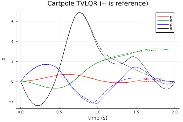
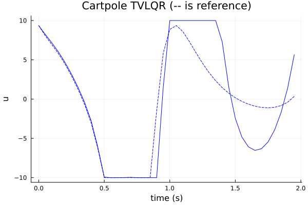
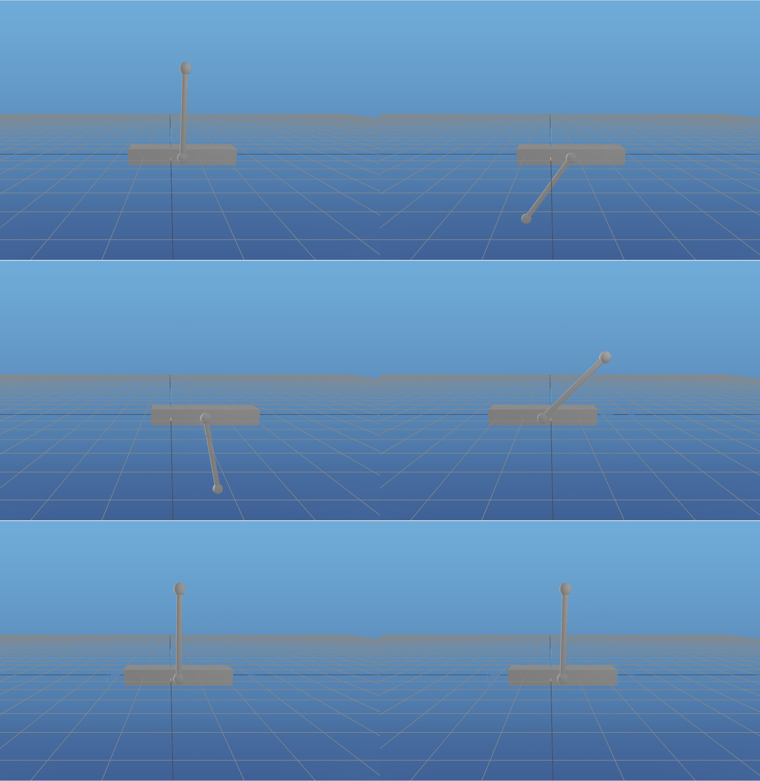
类似HW2 Q2 PartC,使用DIRCOL得到的开环状态轨迹和控制轨迹,通过TVLQR跟踪该轨迹以补偿模型失配。DIRCOL的动力学约束使用了Hermite-Simpson积分方法,但闭环控制使用RK4进行数值积分,并且对闭环控制进行截断(clamp.(U[k],-10,10))防止违约。
HW3_Q2 四旋翼无人机iLQR 示例
使用iLQR求解四旋翼无人机(6DOF)的轨迹优化问题,使用如下特定的代价函数促使无人机完成指定的机动动作(∞)
四旋翼的连续时间动力学模型在 quadrotor.jl中完成,通过rk4进行离散化,四旋翼的状态向量表示如下
其中 是无人机在世界坐标系(N)的位置, 是无人机在世界坐标系(N)的速度(N), 是无人机姿态的修正罗德里格斯参数(Modified Rodrigues Parameter, MRP)表示(即机体坐标系相对于世界坐标系的旋转), 是无人机在机体坐标系的角速度。
补充:MRP使用三个参数表示旋转,在360°会遇到奇点(singularity)但在本次给定的规划动作不会使姿态旋转接近奇点。
include(joinpath(@__DIR__, "utils", "quadrotor.jl"))functiondiscrete_dynamics(params::NamedTuple, x::Vector, u, k) # discrete dynamics # x - state # u - control # k - index of trajectory # dt comes from params.model.dt returnrk4(params.model, quadrotor_dynamics, x, u, params.model.dt)endPart A: iLQR for a quadrotor (25 pts)
iLQR用来解决如下的优化控制问题 :
是初始状态, 是系统离散动力学模型, 是状态代价函数, 是终端代价函数。由于优化问题可以是非凸的,因此不能保证收敛到全局最小值,但实际可以取得良好的效果。
针对此问题,选取如下的状态代价函数和终端代价函数来促使无人机跟踪设定的参考轨迹:
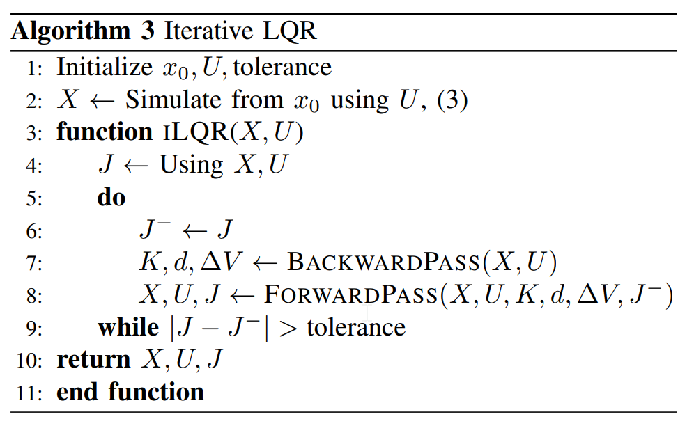
这里需要补充 iLQR的实现过程,用反向传播(backward pass)计算的值函数增量来判断iLQR的收敛,并在solve_quadrotor_trajectory函数中调用。
cost function的实现
# starter code: feel free to use or not use
function stage_cost(p::NamedTuple, x::Vector, u::Vector, k::Int) # TODO: return stage cost at time step k Q, R, xref, uref = p.Q, p.R, p.Xref[k], p.Uref[k] return 0.5 * (x - xref)' * Q * (x - xref) + 0.5 * (u - uref)' * R * (u - uref)endfunction term_cost(p::NamedTuple, x) # TODO: return terminal cost Qf, xref = p.Qf, p.Xref[end] return 0.5 * (x - xref)' * Qf * (x - xref)endfunction stage_cost_expansion(p::NamedTuple, x::Vector, u::Vector, k::Int) # TODO: return stage cost expansion # if the stage cost is J(x,u), you can return the following # ∇ₓ²J, ∇ₓJ, ∇ᵤ²J, ∇ᵤJ Q, R, xref, uref = p.Q, p.R, p.Xref[k], p.Uref[k] Jxx = Q Jx = Q * (x - xref) Juu = R Ju = R * (u - uref) return Jxx, Jx, Juu, Juendfunction term_cost_expansion(p::NamedTuple, x::Vector) # TODO: return terminal cost expansion # if the terminal cost is Jn(x,u), you can return the following # ∇ₓ²Jn, ∇ₓJn
Qf, xref = p.Qf, p.Xref[end] Jn_xx = Qf Jn_x = Qf * (x - xref) return Jn_xx, Jn_xend反向传播(backward pass)
原实现曾在 K[k] 出现 NaN 时直接替换为 K[k+1]。这会掩盖反向递推失败,相邻时刻的增益也不能随意替代,因此已移除。对称标量代价的二阶导数应满足 Qxu = Qux';单独重算交叉项不能证明 NaN 的原因是累计误差。
下面增加有限值检查、对称化和基于 Cholesky 的正定性检查。对称化只适合小幅数值漂移;若不对称误差较大,应追查导数和递推实现。代码仍依赖作业的 discrete_dynamics 等函数,未完成原四旋翼实验复现。
function backward_pass(params::NamedTuple, # useful params X::Vector{Vector{Float64}}, # state trajectory U::Vector{Vector{Float64}}) # control trajectory # compute the iLQR backwards pass given a dynamically feasible trajectory X and U # return d, K, ΔJ
# outputs: # d - Vector{Vector} feedforward control # K - Vector{Matrix} feedback gains # ΔJ - Float64 expected decrease in cost
nx, nu, N = params.nx, params.nu, params.N
# vectors of vectors/matrices for recursion P = [zeros(nx, nx) for i = 1:N] # cost to go quadratic term p = [zeros(nx) for i = 1:N] # cost to go linear term d = [zeros(nu) for i = 1:N-1] # feedforward control K = [zeros(nu, nx) for i = 1:N-1] # feedback gain
# TODO: implement backwards pass and return d, K, ΔJ N = params.N ΔJ = 0.0
P[N], p[N] = term_cost_expansion(params, X[end]) for k = N-1:-1:1 Jxx, Jx, Juu, Ju = stage_cost_expansion(params, X[k], U[k], k)
A_k = FD.jacobian(_x -> discrete_dynamics(params, _x, U[k], k), X[k]) B_k = FD.jacobian(_u -> discrete_dynamics(params, X[k], _u, k), U[k]) @assert all(isfinite, A_k) "A_k has NaN or Inf at step $k" @assert all(isfinite, B_k) "B_k has NaN or Inf at step $k" gx = Jx + A_k' * p[k+1] gu = Ju + B_k' * p[k+1]
Qxx = Jxx + A_k' * P[k+1] * A_k Quu = Juu + B_k' * P[k+1] * B_k Qux = B_k' * P[k+1] * A_k Qxu = Qux'
β = 1e-1 @assert all(isfinite, Quu) && all(isfinite, Qux) && all(isfinite, gu) Quu = (Quu + Quu')/2 F = nothing
for i =1:15 candidate = cholesky(Symmetric(Quu + β*I); check=false) if issuccess(candidate) F = candidate break end β *= 10 end
F === nothing && error("Quu regularization failed at step $k") d[k] = -(F \ gu) K[k] = -(F \ Qux) @assert all(isfinite, d[k]) && all(isfinite, K[k])
p[k] = gx + K[k]' * gu + K[k]' * Quu * d[k] + Qxu * d[k] P[k] = Qxx + K[k]' * Quu * K[k] + Qxu * K[k] + K[k]' * Qux P[k] = (P[k] + P[k]')/2 # α=1 的局部二次模型预测下降;实际下降仍需前向验证。 ΔJ += -(dot(d[k], gu) + 0.5*dot(d[k], Quu*d[k])) end return d, K, ΔJend前向更新(foward pass)
function trajectory_cost(params::NamedTuple, # useful params X::Vector{Vector{Float64}}, # state trajectory U::Vector{Vector{Float64}}) # control trajectory # compute the trajectory cost for trajectory X and U (assuming they are dynamically feasible) N = params.N cost = 0 for i = 1:N-1 cost += stage_cost(params, X[i], U[i], i) end cost += term_cost(params, X[N]) # TODO: add trajectory cost return costend
function forward_pass(params::NamedTuple, # useful params X::Vector{Vector{Float64}}, # state trajectory U::Vector{Vector{Float64}}, # control trajectory d::Vector{Vector{Float64}}, # feedforward controls K::Vector{Matrix{Float64}}; # feedback gains max_linesearch_iters=20) # max iters on linesearch # forward pass in iLQR with linesearch # use a line search where the trajectory cost simply has to decrease (no Armijo)
# outputs: # Xn::Vector{Vector} updated state trajectory # Un::Vector{Vector} updated control trajectory # J::Float64 updated cost # α::Float64. step length
nx, nu, N = params.nx, params.nu, params.N Xn = [zeros(nx) for i = 1:N] # new state history Un = [zeros(nu) for i = 1:N-1] # new control history
# initial condition Xn[1] = 1 * X[1] # initial step length α = 1.0 # TODO: add forward pass #current cost J = trajectory_cost(params, X, U) Jn = trajectory_cost(params, Xn, Un) for i = 1:max_linesearch_iters for k = 1:N-1 Un[k] = U[k] + K[k] * (Xn[k] - X[k]) + α * d[k] Xn[k+1] = discrete_dynamics(params, Xn[k], Un[k], k) end Jn = trajectory_cost(params, Xn, Un) if isfinite(Jn) && Jn < J return Xn, Un, Jn, α else α = 0.5 * α end end error("forward pass failed")endiLQR实现
function iLQR(params::NamedTuple, # useful params for costs/dynamics/indexing x0::Vector, # initial condition U::Vector{Vector{Float64}}; # initial controls atol=1e-3, # convergence criteria: ΔJ < atol max_iters=250, # max iLQR iterations verbose=true) # print logging
# iLQR solver given an initial condition x0, initial controls U, and a # dynamics function described by `discrete_dynamics`
# return (X, U, K) where # outputs: # X::Vector{Vector} - state trajectory # U::Vector{Vector} - control trajectory # K::Vector{Matrix} - feedback gains K
# first check the sizes of everything @assert length(U) == params.N - 1 @assert length(U[1]) == params.nu @assert length(x0) == params.nx
nx, nu, N = params.nx, params.nu, params.N # TODO: initial rollout X = [x0 for i = 1:N] for i = 1:N-1 X[i+1] = discrete_dynamics(params, X[i], U[i], i) end
for ilqr_iter = 1:max_iters d, K, ΔJ = backward_pass(params, X, U) # 只在有限、非负的预测下降足够小时停止;不能将负值当作收敛。 if isfinite(ΔJ) && 0 <= ΔJ < atol if verbose @info "iLQR converged" end return X, U, K end Xn, Un, J, α = forward_pass(params, X, U, d, K) X, U = Xn, Un
# ---------------logging ------------------- if verbose dmax = maximum(norm.(d)) if rem(ilqr_iter - 1, 10) == 0 @printf "iter J ΔJ |d| α \n" @printf "-------------------------------------------------\n" end @printf("%3d %10.3e %9.2e %9.2e %6.4f \n", ilqr_iter, J, ΔJ, dmax, α) end
end error("iLQR failed")end给出参考轨迹和控制,定义模型参数
function create_reference(N, dt) # create reference trajectory for quadrotor R = 6 Xref = [ [R*cos(t);R*cos(t)*sin(t);1.2 + sin(t);zeros(9)] for t = range(-pi/2,3*pi/2, length = N)] for i = 1:(N-1) Xref[i][4:6] = (Xref[i+1][1:3] - Xref[i][1:3])/dt end Xref[N][4:6] = Xref[N-1][4:6] Uref = [(9.81*0.5/4)*ones(4) for i = 1:(N-1)] return Xref, Urefendfunction solve_quadrotor_trajectory(;verbose = true)
# problem size nx = 12 nu = 4 dt = 0.05 tf = 5 t_vec = 0:dt:tf N = length(t_vec)
# create reference trajectory Xref, Uref = create_reference(N, dt)
# tracking cost function Q = 1*diagm([1*ones(3);.1*ones(3);1*ones(3);.1*ones(3)]) R = .1*diagm(ones(nu)) Qf = 10*Q
# dynamics parameters (these are estimated) model = (mass=0.5, J=Diagonal([0.0023, 0.0023, 0.004]), gravity=[0,0,-9.81], L=0.1750, kf=1.0, km=0.0245,dt = dt)
# the params needed by iLQR params = ( N = N, nx = nx, nu = nu, Xref = Xref, Uref = Uref, Q = Q, R = R, Qf = Qf, model = model )
# initial condition x0 = 1*Xref[1]
# initial guess controls U = [(uref + .0001*randn(nu)) for uref in Uref]
# solve with iLQR X, U, K = iLQR(params,x0,U;atol=1e-4,max_iters = 250,verbose = verbose)
return X, U, K, t_vec, paramsend结果(迭代过程,位置,速度,姿态,角速度和控制量变化)
iter J ΔJ |d| α------------------------------------------------- 1 2.988e+02 1.37e+05 2.88e+01 1.0000 2 1.075e+02 5.31e+02 1.35e+01 0.5000 3 4.903e+01 1.33e+02 4.73e+00 1.0000 4 4.429e+01 1.15e+01 2.48e+00 1.0000 5 4.402e+01 8.05e-01 2.51e-01 1.0000 6 4.398e+01 1.44e-01 8.32e-02 1.0000 7 4.396e+01 3.78e-02 7.28e-02 1.0000 8 4.396e+01 1.29e-02 3.76e-02 1.0000 9 4.396e+01 5.06e-03 3.19e-02 1.0000 10 4.396e+01 2.28e-03 1.94e-02 1.0000iter J ΔJ |d| α------------------------------------------------- 11 4.396e+01 1.14e-03 1.61e-02 1.0000 12 4.395e+01 6.21e-04 1.09e-02 1.0000 13 4.395e+01 3.62e-04 8.94e-03 1.0000 14 4.395e+01 2.22e-04 6.61e-03 1.0000 15 4.395e+01 1.40e-04 5.39e-03 1.0000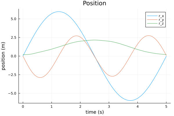
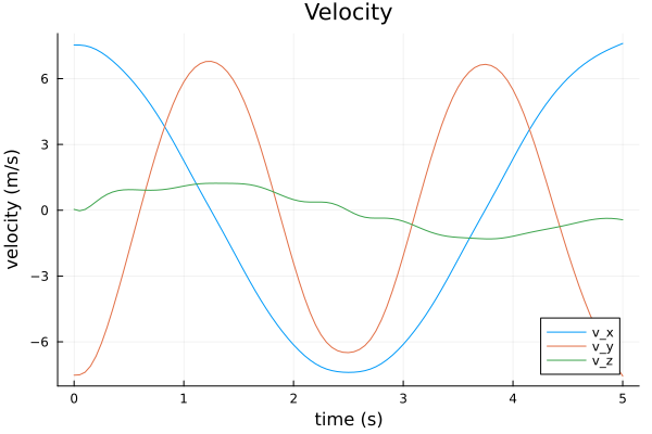
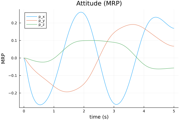
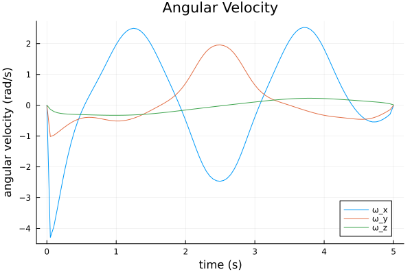
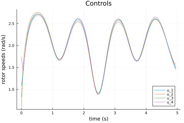
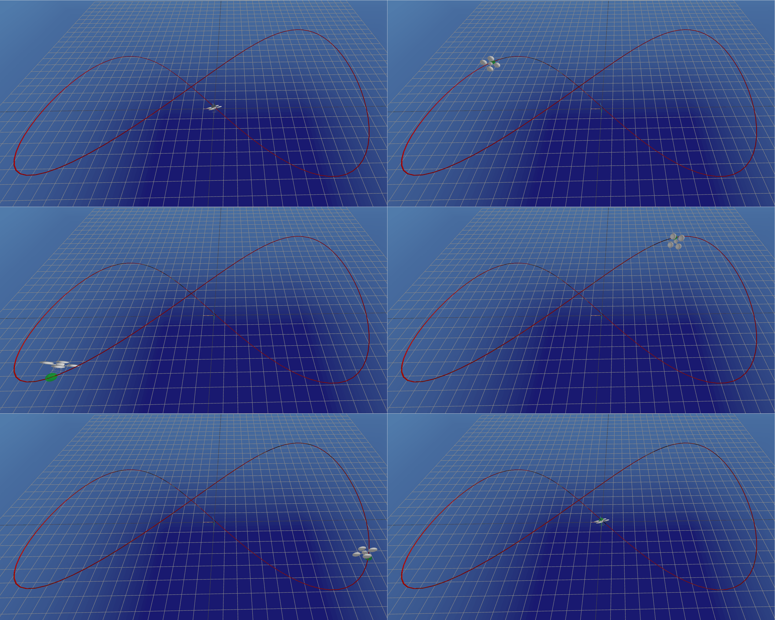
Part B
通过iLQR生成的轨迹是开环,实际中会因模型误差(如风扰、参数不准)而偏离,这里使用iLQR得到的参考轨迹和时变增益矩阵获得TVLQR反馈控制(注意K的正负号,这里输出的k=-Quu\Qux,自带了负号)
# set verbose to false when you submit Xilqr, Uilqr, Kilqr, t_vec, params = solve_quadrotor_trajectory(verbose = false)
# real model parameters for dynamics model_real = (mass=0.5, J=Diagonal([0.0025, 0.002, 0.0045]), gravity=[0,0,-9.81], L=0.1550, kf=0.9, km=0.0365,dt = 0.05)
# simulate closed loop system nx, nu, N = params.nx, params.nu, params.N Xsim = [zeros(nx) for i = 1:N] Usim = [zeros(nu) for i = 1:(N-1)]
# initial condition Xsim[1] = 1*Xilqr[1]
# TODO: simulate with closed loop control
for i = 1:(N-1) Usim[i] = Uilqr[i]+Kilqr[i]*(Xsim[i]-Xilqr[i]) Xsim[i+1] = rk4(model_real, quadrotor_dynamics, Xsim[i], Usim[i], model_real.dt) endTVLQR结果如下
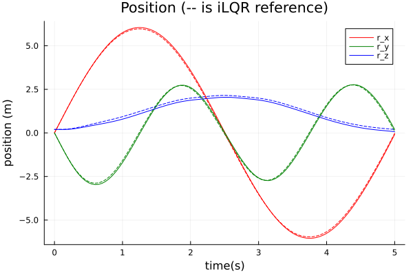
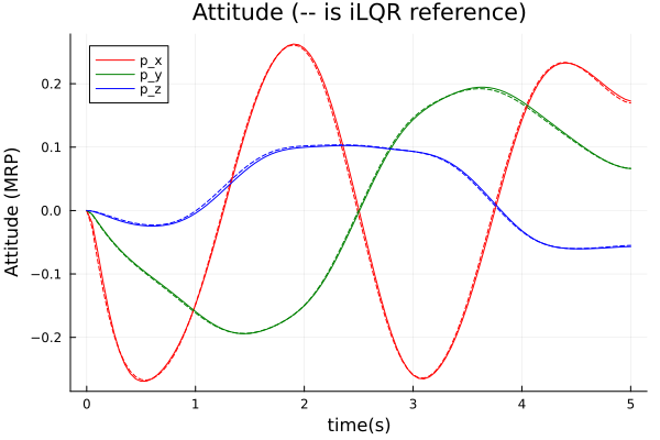
HW3_Q3
问题要求
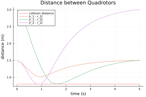
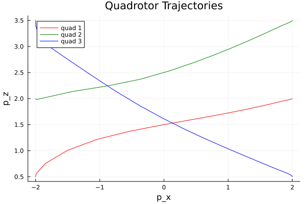
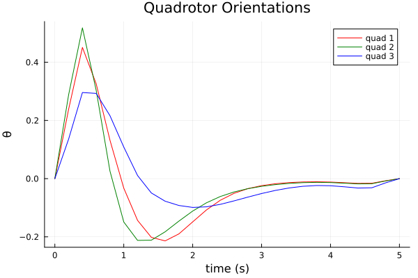
实现三架平面无人机的无碰撞的轨迹优化问题,要求如下
- 无人机的初始位置和末端期望位置给定
- 无人机彼此的距离不能小于
一般的iLQR无法直接处理碰撞约束,需要在代价函数中纳入距离成本,但无法保证完全满足距离约束,这里选择使用直接配点法DIRCOL,求解问题的数学形式设计如下
实际中将三架无人机各自的状态变量和控制变量进行合并,为整个要求解的优化变量
碰撞约束可写成 ,代码用 sum(abs2, p_i-p_j),直接表达平滑的平方距离,避免先计算零点不可微的 norm 再平方。该约束是非凸的,且只在离散节点满足距离下限不足以保证节点之间或有尺寸的无人机无碰撞;还需加密轨迹验证并纳入几何尺寸。
初始轨迹的生成可以使用 x_initialize = range(xic, xg, length = N)
整体的代码框架与HW3_Q1基本一致,结果如下
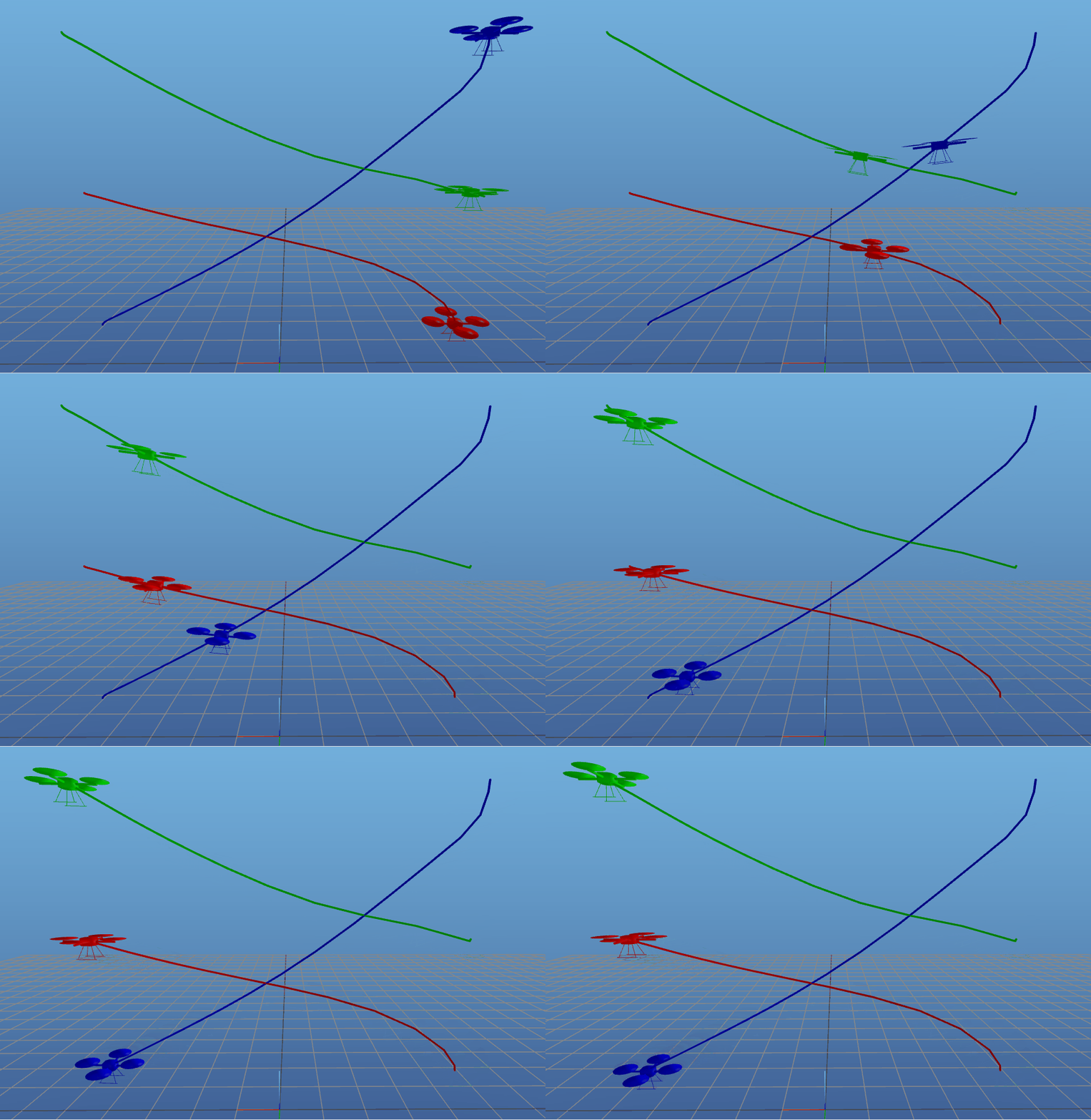
整理与核查说明
本笔记原有许可为 CC BY 4.0。引用的课程材料、代码和图片仍须遵守其各自的许可。
核查状态:部分验证(2026-10-04)。 Julia 1.10.10 的简化线性测试检验 iLQR 递推与线搜索拒绝逻辑;原四旋翼和 DIRCOL 实验待复现。
2026-10-04 整理时修正了已定位的公式和实现问题。文中的图片、动画和输出保留自学习时的实验记录,不代表修订后的代码已经完整重跑。作业片段依赖原项目环境,不能直接作为完整可运行教程;具体核查范围与尚未复现事项见正文。
分享文章
生成精美分享图或复制链接,与更多人分享本文。
继续阅读
最后更新于 ,距今已过 0 天
部分内容可能已过时